S01 · Slow the language model down 00:00–01:30
Audience takeaway A language model repeatedly predicts possible next tokens from the available context.
Speaker beats Introduce the question: how can next-token prediction produce useful language? Given Alice was, compare beginning at 60%, getting at 25%, and very at 15%. The percentages and bar lengths show how likely each candidate is in this example. The red word is selected; advance so it joins the context. The updated context produces a fresh distribution. Keep advancing one word at a time until the sentence is complete. The same model is reused. The following scenes unpack tokens, representations, attention, training, and generation.
Keep the explanation precise The alternatives, probabilities, and selections are scripted illustrations, not a live model. Each simplified three-choice distribution sums to 100%; a real model scores its entire vocabulary. This preview selects the most likely candidate; sampling from the distribution comes later. Words stand in for tokens; actual token boundaries vary. Generation holds the trained weights fixed.
Transition Start with a prediction everyone can make.
From Grokking AI Algorithms, Second Edition Figure 11.3 · printed page 390 · PDF page 422 S02 · Ask the room what comes next 01:30–03:00
Audience takeaway Generation starts with a distribution over possible continuations.
Speaker beats Ask the room what could follow Hey, what are. Advance to reveal the candidates, then compare you, we, and the. The highlighted word is the immediate next-token choice. The grey continuation shows where that choice could lead; it is illustrative future text, not a claim about a real model’s predictions.
Keep the explanation precise Do not attach invented model probabilities to the phone suggestions.
Transition How could we learn even this tiny prediction task?
From Grokking AI Algorithms, Second Edition Figure 11.1 · printed page 388 · PDF page 420 S03 · Build a tiny predictor from counts 03:00–06:00
Audience takeaway Counts give us a useful starting point, but a bigram remembers only one previous token.
Speaker beats Start with the book’s five training sentences. Advance to highlight the first Alice → was pair as it travels into the count table. Advance again for the second Alice → was, then the Alice → and in the last sentence. Keep the text and table in place while the counts build. Next reveal the denominator of three, then the percentages and bars: 2/3 is about 66.7%, 1/3 about 33.3%. Compare the completed row for was. Then show The White Rabbit: Rabbit is followed by was twice and were once in the same training text, so the model assigns 66.7% and 33.3%. Advance to add Alice and the Rabbit. The model still favours was because only Rabbit selects the row; it cannot use the earlier words to recognise the plural subject. The candidates have different probabilities, but both contexts receive the same distribution. Advance to ask how a model could use more context. Only now introduce the architecture map: represent the text, mix its context in repeated blocks, then predict a next token. Spend about 30 seconds tracing the forward path and the append-and-repeat loop. Name the parts without teaching them yet; the map will return before each close-up.
Keep the explanation precise Modern LLMs are neural predictors, not large lookup tables of bigram counts. Keep these toy counts tied to the five sentences. The architecture map is simplified from the book’s decoder-style model. Additive sinusoidal positions are shown; residual connections and layer normalization are omitted from the audience view, not from the actual model. These details vary across models. Tokenization and selection surround the learned model. The last position supplies the next-token prediction during generation; training can score all positions in parallel.
Transition We now have the map. Begin at its input: what counts as a token?
From Grokking AI Algorithms, Second Edition Figure 11.3 · printed page 390 · PDF page 422 Figure 11.5 · printed page 392 · PDF page 424 S04 · Text becomes tokens, then IDs 06:00–09:00
Audience takeaway A token is a vocabulary item; it is not necessarily a whole word.
Speaker beats First show the full normalized training paragraph. Advance to put every character in its own box, including spaces and punctuation. The space symbol stands for a space character, not a literal new character in the text. The enlarged excerpt below shows the same individual characters. Next return to the book’s within-word merge exercise, where </w> marks a word boundary. The tokenizer learns merge rules from training text, not only from the short sentence we want to encode. Figure 11.14 supplies the full normalized passage shown here. Count i+n twice in beginning and once in sitting, having, nothing, into, reading, and the standalone word in: eight total. Our short excerpt contains only the two in beginning; the remaining six come from elsewhere in the passage. After learning i+n -> in, apply the rule in the excerpt. Repeated counting and merging over the training text leads to further rules. The later in, ic, and ing highlights show selected learned pieces in the passage; the illustrated rule list is not the full merge history. Finally, the vocabulary excerpt maps each token to the IDs in table 11.6. Identical tokens share an ID.
Keep the explanation precise The passage and source counts are grounded in figure 11.14 and the i+n row of table 11.3. Count adjacent letters within words, retaining the distinction between training text and the shorter excerpt. Only selected merge rules and vocabulary entries are displayed; do not imply that these are a complete learned tokenizer or that the full vocabulary follows from one merge. This toy character-based example does not reproduce every production tokenizer. The added full-character view preserves every character of the normalized passage. It is the starting representation in this teaching example, not a claim that all modern tokenizers use Unicode characters as their base units.
Transition An integer ID is an address. What does it look up?
From Grokking AI Algorithms, Second Edition Figure 11.14 · printed page 402 · PDF page 434 Figure 11.19 · printed page 408 · PDF page 440 S05 · Look up a learned representation 09:00–11:00
Audience takeaway Embeddings turn discrete vocabulary items into numeric representations that training can shape.
Speaker beats Use the first 5–10 seconds to locate the highlighted component on the familiar architecture map, then advance into the close-up. The ID is an address, not a numeric feature from which we calculate meaning. Select a, l, and b and point to their stored rows. Each of the four coordinates is a trainable parameter. Start with small random values; training adjusts them to improve next-token predictions. We will explain those updates in the training section. At generation time the table is fixed and we simply look up the row. Individual coordinates have no predefined semantic labels. Return to the architecture map to highlight position and addition before connecting WHAT token and WHERE it occurs: the book adds a learned token vector and a position vector. Keep the same a at position 0 for the next section.
Keep the explanation precise The displayed rows come from table 11.8. They are examples of stored parameters, not numbers calculated from the token ID. Do not claim every row matches an earlier initialization range. This toy uses four dimensions and additive sinusoidal positions; other architectures can encode position differently.
Transition We also need to tell the model where each token occurs.
From Grokking AI Algorithms, Second Edition Figure 11.28 · printed page 418 · PDF page 450 S06 · Order changes meaning 11:00–12:30
Audience takeaway Position gives attention access to token order.
Speaker beats Keep the token sequence from the book visible and point to a at positions 0 and 5. Both occurrences look up the same learned embedding. Advance to add their different position vectors, coordinate by coordinate. Then switch to dog bites man: the red bars represent token embeddings, the blue bars represent position codes, and the grey bars represent their sums. Advance to swap dog and man. Each word carries its unchanged embedding to its new place, while the position codes stay attached to positions 0, 1, and 2. The grey inputs change because each moved word is combined with a different position code. Order changes meaning, so the model needs information about both identity and position. We do not need to derive the code to understand its purpose.
Keep the explanation precise The bar patterns show four signed coordinates on a shared scale; the grey bars are actual coordinate-wise sums. The dog, bites, and man embeddings are constructed teaching values, not trained model parameters. Words stand in for tokens. The position codes still use the book’s additive sinusoidal example, but the trigonometric derivation is omitted. Position depends on the slot, not the word. Four dimensions are for illustration. Modern architectures can encode position differently, for example through rotary encoding inside attention. Adding position supplies information; it does not by itself interpret sentence meaning.
Transition We now represent both token identity and position. Attention can use those representations to gather context.
From Grokking AI Algorithms, Second Edition Figure 11.29 · printed page 420 · PDF page 452 S07 · Attention mixes information from context 12:30–14:00
Audience takeaway A token can form a context-dependent representation by weighting information from other tokens.
Speaker beats Use the first 5–10 seconds to locate the highlighted component on the familiar architecture map, then advance into the close-up. Attention computes a weighted mixture of value vectors. It helps information flow between positions. The link to Alice is intuition for context use, not a claim that one attention head reliably solves pronouns.
Keep the explanation precise Use no fake measured scores. Attention weights are not proof of reasoning, causality, or a faithful explanation.
Transition How are those weights and mixtures computed?
S08 · Queries, keys, and values 14:00–18:00
Audience takeaway Queries match keys; the resulting weights mix values.
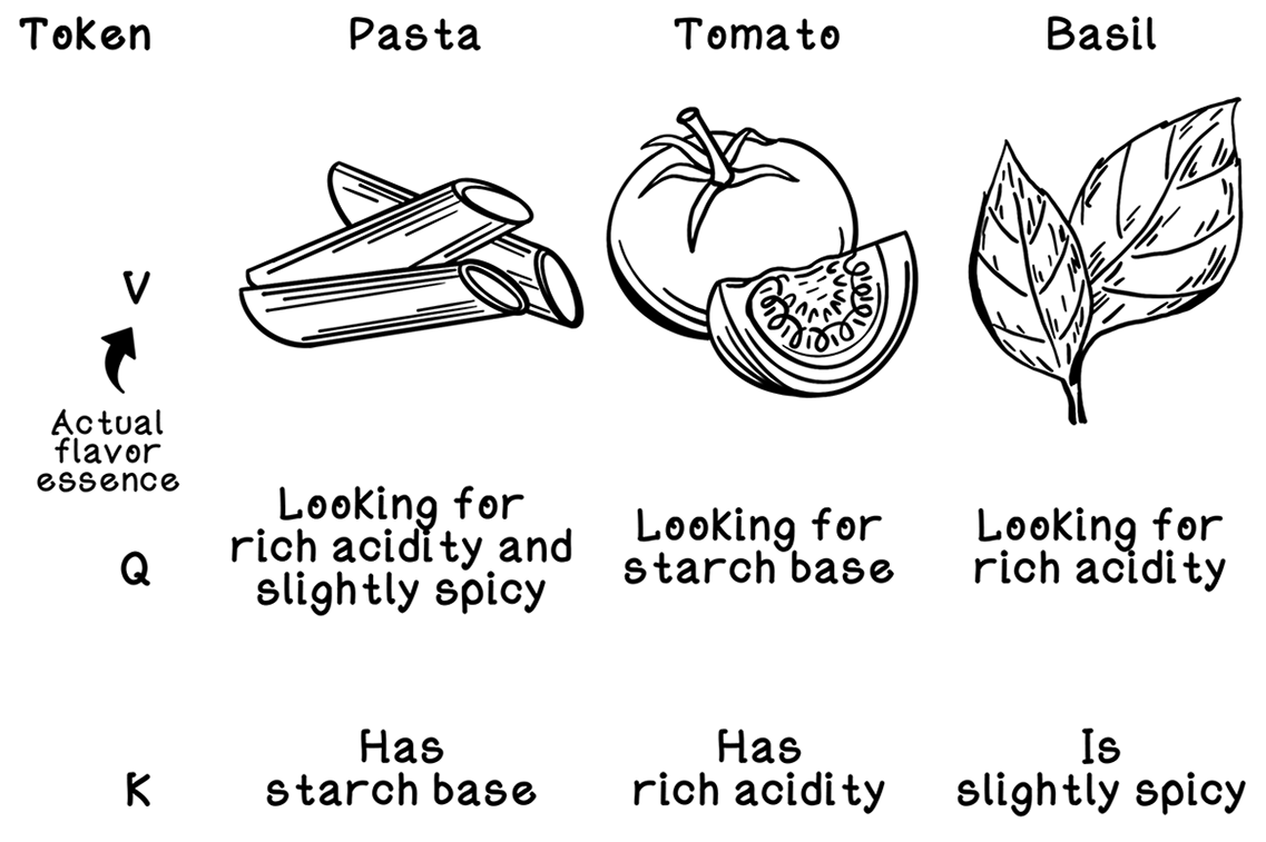
Speaker beats Keep the roles distinct: query asks, keys are compared, and values are mixed. The words and drawings are the book’s analogy, while the percentages are calculated from a small illustrative vector example. Choose rich acidity, starch, and slight spice to see the weights change without changing the available values. Role letters and names accompany every colour; ingredient colours identify the separate values in the mixture. After the pantry analogy, apply exactly these roles to the sentence: the query at she compares with keys from the same sequence and mixes its available values. That shared source is why it is called self-attention. Keep the masking rule on the sentence itself: earlier positions and the current position are available; future positions are faded and have weight zero. Advance directly from the pantry to the sentence with its weighted values, without separate sequence-reading or matrix slides. Direct connections make distant context accessible, and training can process the positions in parallel while respecting the mask.
Keep the explanation precise The actual Q/K/V entries are learned vectors, not ingredient labels. Masking must happen before softmax. Leave matrix arithmetic to optional Q&A. The sentence weights are illustrative, not measured model explanations or proof of coreference. Words stand in for tokens in this close-up. Parallel training does not make autoregressive generation parallel.
Transition That is one way to gather context. Several heads learn different ways to do it.
From Grokking AI Algorithms, Second Edition Figure 11.34 · printed page 426 · PDF page 458 S09 · Several heads, several learned views 18:00–20:00
Audience takeaway Multiple heads can mix information in different ways before their outputs are combined.
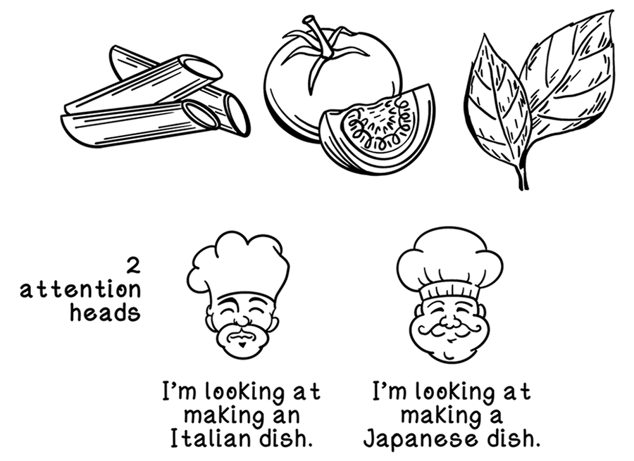
Speaker beats Use the first 5–10 seconds to locate the highlighted component on the familiar architecture map, then advance into the close-up. Keep the book’s chefs-and-pantry metaphor, now give each chef a dish to aim for. Both see flour, tomato, cheese, and basil. Chef 1 wants an Italian-style dish, illustrated as tomato-and-basil pasta. Chef 2 wants a New York-style dish, illustrated as pizza. Compare their attention patterns: each mixes information from several ingredients, with different emphasis. The percentages describe attention, not recipe quantities. Each head has its own learned query, key, and value projections. On the third chef advance, keep both coloured output strips side by side: concatenate the head outputs, then apply a learned output projection to make one richer representation. This combines information from both views; it does not choose a winning chef. Then switch to Alice gave Bob a red book. Keep the query position fixed at book and reveal three illustrative heads: giver, recipient, and colour. Each head assigns nonzero weights to several words, but their strongest weights fall on Alice, Bob, and red respectively. One head can already read multiple positions; the benefit here is independent attention weights and value projections, with separate output vectors h1, h2, and h3 before concatenation and the learned output projection. These are possible teaching perspectives, not discovered head assignments. Real heads learn their patterns jointly from data and are not assigned cuisines or guaranteed specialities. Spend about one minute on the chefs and one minute on the sentence. Reference for the parallel-head mechanism: https://arxiv.org/abs/1706.03762, section 3.2.2.
Keep the explanation precise The dishes, pantry, and normalized attention weights are constructed illustrations, not authentic recipes or measured model heads. One-hot ingredient values make the output blends easy to follow. The final projected bars are schematic. Chefs stand for parallel learned projections, not independent agents; human-readable specialities are not guaranteed. The sentence weights and giver/recipient/colour labels are constructed illustrations, not measured model behavior. Words stand in for tokens. All shown positions are available to the causal query at book. Percentages are attention weights, not next-token probabilities. h1, h2, and h3 represent weighted sums of each head’s own projected value vectors; they are not the selected words. No claim is made that a single head could never solve the task.
Transition Attention mixes information between tokens. Next, a feed-forward network transforms the features at each position.
From Grokking AI Algorithms, Second Edition Figure 11.40 · printed page 436 · PDF page 468 S10 · Transform each token with a neural network 20:00–22:30
Audience takeaway A feed-forward network transforms each position’s features using learned weights and a nonlinear activation.
Speaker beats Use the first 5–10 seconds to locate the highlighted component on the familiar architecture map, then advance into the close-up. First show the biological neuron, following the supplied screenshot and page 32 of the Porto primer. Name the dendrites, cell body or soma, nucleus, axon, and synaptic contacts. Trace incoming signals toward the cell body and outgoing signaling along the axon to contacts with other cells. The brief signal animation suggests direction only. Use this as the intuition for gathering inputs and producing an output; advance to the mathematical neuron. Before the driving network, spend about 35 seconds on the single-neuron diagram adapted from the Porto primer, PDF pages 33–34 and 41. Start with exactly its four inputs (0.15, 0.5, 0.7, 0.22) and four weights (0.22, 0.27, 0.72, 0.05). Advance to show their products: 0.033, 0.135, 0.504, 0.011. Add them to get 0.683; bias is zero in this example. Advance to apply the step activation: a nonnegative sum gives 1, a negative sum gives 0. The output 1 is a binary activation, not a probability. The two halves of the large circle are operations inside the same neuron, not two hidden neurons. Now connect many such units into a network. The driving example changes the inputs and uses ReLU in its hidden neurons and sigmoid at its output; the common computation is a weighted sum plus bias followed by an activation. Start with the driving example from the Porto primer, PDF pages 48–50: 40 mph, terrain 5/10, visibility 180 degrees, and 50k miles driven. Divide by the original ranges of 70, 10, 360, and 300k to get four scaled inputs. Keep the network visible while three hidden neurons combine different pairs: speed and terrain, speed and visibility, and terrain and distance driven. Their coloured connections match the nonzero weights; the dotted connections have weight zero. Walk through one calculation, then compare the other two weighted sums and ReLU outputs: 0.471, 0.271, and 0.067. On the next advance, combine those activations into the sigmoid collision output of 59.6%. These weights are constructed to explain the computation, not taken from a trained collision predictor. Unlike the old primer, this teaching close-up uses three hidden ReLU neurons. Briefly connect this computation back to the highlighted FFN: a Transformer transforms each position’s context-aware features using shared learned weights. Its FFN returns features, while a separate vocabulary projection after the last block supplies token scores. Keep the driving network visible and ask how its weights are learned; advance directly into the training example.
Keep the explanation precise This is a compact 4-to-3-to-4 teaching network, not a complete Transformer or the book’s wider 4-to-16-to-4 FFN. The four input values are shared with the embedding-plus-position example; they are reused to illustrate network arithmetic rather than claimed to be a computed attention output. The FFN returns four features; the separate head produces probabilities over three example tokens. Weights and biases are illustrative, with head biases initialized to the chosen starting distribution. All values and updates are computed by the same model, and every parameter gradient is checked numerically. The backward overlay highlights one route while calculations include all paths. Lower loss on this single example does not establish generalization. The driving inputs and scaling ranges come from the Porto primer; the weights, ReLU hidden layer, and output probability are newly constructed teaching values. This is not a validated collision model. The named pairs are constructed for teaching, with other incoming weights set to zero. Real hidden neurons learn mixtures of inputs; they are not assigned guaranteed human-readable roles. Distance driven is used as an experience-related input in this illustration. The driving example uses a sigmoid prediction head; the Transformer FFN returns features without that head. The single-neuron example reproduces the primer’s numbers with decimal points. Its step activation is the classic perceptron rule, with bias 0; modern Transformer FFNs use other activations. The arbitrary inputs on this first diagram are not the normalized driving measurements on the following diagram. Learning is demonstrated in the next section. The biological diagram is schematic. Synapses are junctions between cells; faint receiving membranes are included at the axon terminals. The nucleus supports cellular functions and is not the component that calculates a weighted sum or triggers a step activation. A perceptron is a highly simplified mathematical abstraction, not a detailed biological neuron. The pulse animation is not a simulation of membrane dynamics or firing timing.
Transition We can now follow the numbers through a network. How does it learn the weights?
From Grokking AI Algorithms, Second Edition Figure 11.3 · printed page 390 · PDF page 422 S11 · Training learns from the next token 22:30–26:00
Audience takeaway Training changes parameters; the next-token objective supplies many examples from ordinary text.
Speaker beats Use a small four-input neural network to demonstrate learning, with a separate vocabulary head. For this compact numerical example, reuse a’s embedding plus position 0 as the fixed input; the full Transformer would supply context-aware features. It starts with probabilities 12%, 68%, and 20% for l, ic, and e. The training text supplies l as the next token. Loss = -log p(l): assigning low probability to the observed token creates a larger error. Backpropagation calculates how each parameter affects that error. Highlight the x1 connection with gradient 0.424011: at learning rate 0.1 its weight changes from 1 to 0.9575989. Update all weights and biases, run the same example again, and observe the changed activations and probabilities. Six updates bring p(l) to about 94.1% and loss to about 0.06. In the full language model, the same idea also trains embeddings, attention projections, and the other learned parameters across many sequences. Training can score many next-token targets in parallel with a causal mask. The input vector stays fixed in this compact demonstration. Spend the final 45 seconds zooming out to Meta’s published Llama 3.1 405B model. Advance: our four coordinates become 16,384 numbers for every token, 4,096 times wider. Each dot in the square is one coordinate; the square is simply a way to lay out one vector, not an image. Advance: one block has 128 query attention heads and a gated FFN whose intermediate width is 53,248. The FFN returns to the model width of 16,384. Its dots now group 512 coordinates each so the size difference remains visible. Advance: all 126 blocks are shown, each with attention and an FFN and each with its own weights. The model has about 405 billion learned parameters in total. Connect this directly to training: the small weight changes we just followed happen across this enormous collection of weights. Then recap the complete architecture before generating with the learned weights held fixed.
Keep the explanation precise This is a compact 4-to-3-to-4 teaching network, not a complete Transformer or the book’s wider 4-to-16-to-4 FFN. The four input values are shared with the embedding-plus-position example; they are reused to illustrate network arithmetic rather than claimed to be a computed attention output. The FFN returns four features; the separate head produces probabilities over three example tokens. Weights and biases are illustrative, with head biases initialized to the chosen starting distribution. All values and updates are computed by the same model, and every parameter gradient is checked numerically. The backward overlay highlights one route while calculations include all paths. Lower loss on this single example does not establish generalization. Scale figures come from The Llama 3 Herd of Models, Table 3 (Meta, 2024), for the 405B model released as Llama 3.1. They are an example, not a specification for all LLMs. The 128 heads are query heads; grouped-query attention shares 8 key/value heads. This real model uses gated SwiGLU FFNs and rotary positions, so it is not a literal enlargement of the earlier ReLU/additive-position toy. Dimensions count coordinates, blocks count repeated layers, and parameters count learned scalar weights across the full model, including embeddings and the output projection. The FFN drawing summarizes width: it omits the separate gating projection and samples connections, rather than showing all weights. The 16,384-dot field, 128 head tiles, and 126 block tiles have exact counts. The FFN input/output columns contain 32 dots and its intermediate column 104, each representing 512 coordinates.
Transition After training at this scale, hold the learned weights fixed. Trace one prediction through the whole architecture, then use it to generate an answer.
From Grokking AI Algorithms, Second Edition Figure 11.3 · printed page 390 · PDF page 422 Real model dimensions: Meta: The Llama 3 Herd of Models, Table 3
S12 · Recap the architecture, then generate 26:00–31:30
Audience takeaway Autoregressive generation reuses fixed weights on a growing context.
Speaker beats Training has learned the weights. Hold them fixed and recap one prediction using exactly the same architecture map as the close-ups. Advance the highlight through five jobs: represent tokens and positions; mix context with self-attention, including Q/K/V and multiple heads inside that one component; transform each position with the feed-forward network; repeat the block with its own learned weights; project the final last-position vector and use softmax to predict a next token. The audience diagram omits residual connections and layer normalization. If asked, residuals add a sublayer input back to its output, and layer normalization rescales each position’s coordinates. Spend about a minute reconnecting these familiar pieces. Then select a token, append it, and run the same model again in the generation example. Reconnect this to the opening Alice example. Sample twice, then pause at Alice was beginning to. All temperature comparisons and the live demo use the same four illustrative logits: get 4, feel 2, explore 1, dream 0. Temperature divides these scores before softmax. At T=1 the probabilities are about 83.1%, 11.2%, 4.1%, and 1.5%. At T=0.2, get receives more than 99.9%; the others are still possible, but each has less than 0.1%. At T=4, the distribution spreads to about 40.9%, 24.8%, 19.3%, and 15.0%. Keep all three distributions side by side, with the same token colours and a common 0–100% bar scale. Token ranking is unchanged. On the next advance use the same seeded uniform draw, about 0.721, in each distribution: low and original temperature select get; high temperature selects explore. This controlled draw illustrates changed odds, not a guarantee that every high-temperature sample differs. Continue at T=4 and append exactly that explore. The next context offers Wonderland, the, and again. Advance directly to the completed sequence: the remaining draws append Wonderland and the stop symbol. The separate Wonderland-only stop has been removed. This tiny continuation table is a constructed illustration, not a trained Transformer. Temperature does not retrain the model, add knowledge, or guarantee truth.
Keep the explanation precise Use the book’s post-norm ordering consistently. Residuals add vectors of matching width. The FFN weights are shared across positions within a block, while separate blocks have their own parameters. Architectures vary in normalization and position schemes. Vocabulary scores are unnormalized logits; softmax produces token probabilities. Model probabilities describe token likelihood under the model, not confidence that a statement is true. Do not show precise production-model values without running that model. For positive temperature, probabilities are softmax(logits / T); token ranking is unchanged. Lower temperature sharpens unequal scores and higher temperature flattens them. A finite positive temperature does not make the lower-scored token impossible. Greedy selection is a separate choice and is unaffected by positive temperature. The three comparisons use identical context, candidate scores, and model weights. The sampling preview consumes no token; the next advance reconstructs and appends exactly that draw at the same temperature. New bars after appending belong to the new context, not to a different temperature. These four candidates are a teaching example; a real vocabulary is much larger.
Transition That is the loop behind a talking machine. Understanding it gives us a foundation to use and build with these models.
From Grokking AI Algorithms, Second Edition Figure 11.1 · printed page 388 · PDF page 420 S13 · Use them better. Build on them. 31:30–33:00
Audience takeaway You now know how LLMs work. At the very least, use them better. At the most, build on them.
Speaker beats You now know how LLMs work: how text becomes tokens and vectors, how attention and feed-forward networks transform them, how training adjusts the weights, and how generation predicts one token at a time. Pause on that understanding. Advance: my hope is that, at the very least, it helps you use them better. Advance again: at the most, it gives you a foundation to build on them. Let that invitation land before previewing the next talk.
Keep the explanation precise Avoid a blanket claim that these models cannot reason, memorize, count, or retrieve. Describe the missing guarantees and the checks needed.
Transition There is another part of generative AI to explore next.
S14 · Next: Dreaming in Pixels 33:00–33:30
Audience takeaway Beneath Generative AI: Dreaming in Pixels explores how noise becomes an image.
Speaker beats The companion talk is Beneath Generative AI: Dreaming in Pixels. Tease the question: how does noise become an image? I will likely give it at a meetup later this month. The meetup and date are not confirmed yet. Keep this as a brief invitation, then move to the book and projects.
Keep the explanation precise The three 8×8 grids are an illustrative refinement of the book’s happy face, not output from a trained diffusion model. The meetup timing is tentative; no venue or date has been announced.
Transition If you want to keep exploring these algorithms, the book is a place to start.
S15 · Grokking AI Algorithms 33:30–34:00
Audience takeaway Keep exploring the algorithms, build with Viszen, and join the AIZA community.
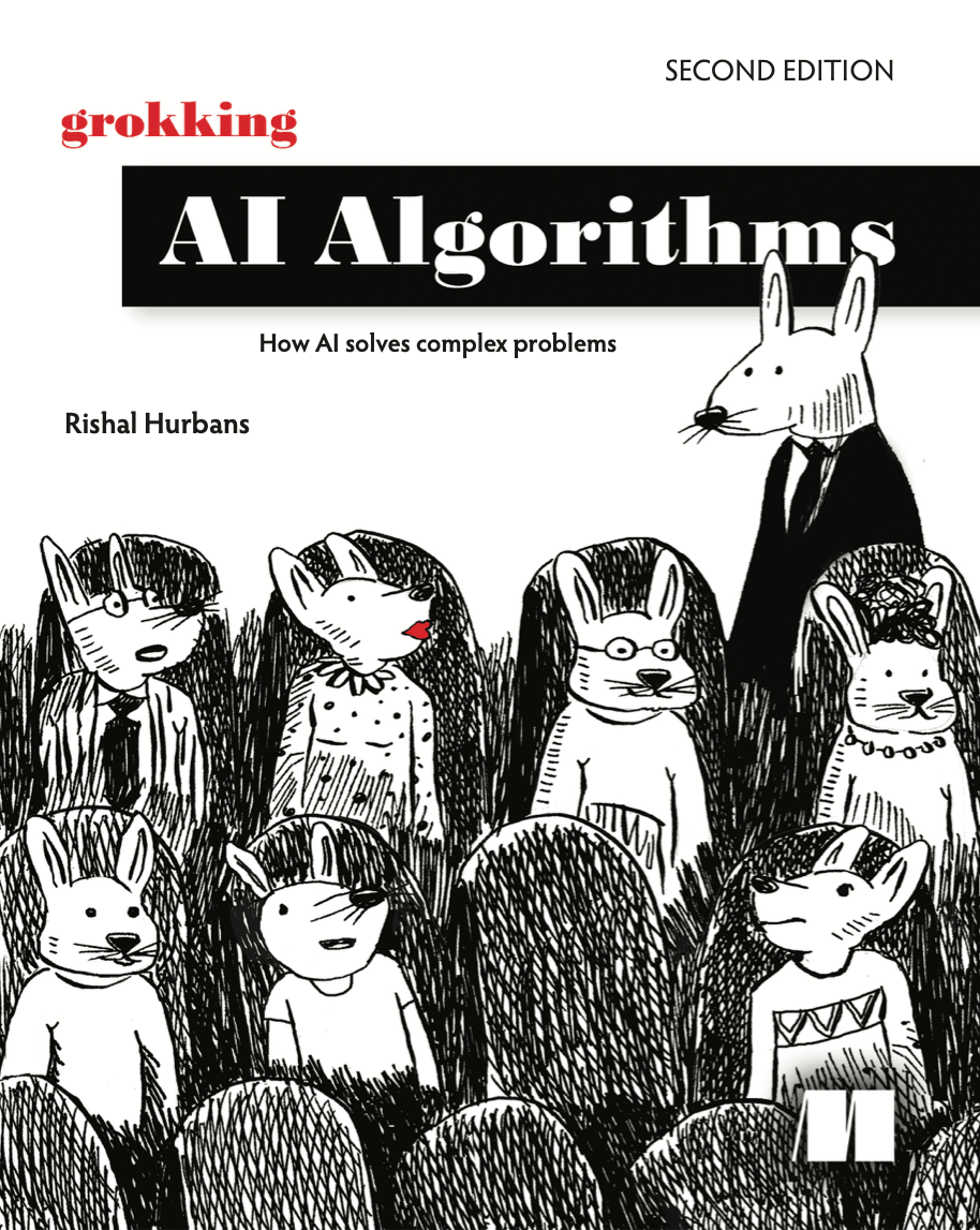
Speaker beats For a deeper visual guide to the algorithms, point to the book and its QR code. Pause before advancing to AIZA.
Keep the explanation precise The QR codes encode the same direct URLs as the links: the book website, Viszen, and AIZA. They are embedded in the offline show; visiting their destinations requires an internet connection.
Transition Questions and conversation.
S16 · AIZA 34:00–34:30
Audience takeaway Keep exploring the algorithms, build with Viszen, and join the AIZA community.
Speaker beats Invite the audience to join the AIZA community for practical AI talks, demos, and conversations. Pause on its QR code, then advance to Viszen.
Keep the explanation precise The QR codes encode the same direct URLs as the links: the book website, Viszen, and AIZA. They are embedded in the offline show; visiting their destinations requires an internet connection.
Transition Questions and conversation.
S17 · Viszen 34:30–35:00
Audience takeaway Keep exploring the algorithms, build with Viszen, and join the AIZA community.
Speaker beats Introduce Viszen and invite the audience to explore how the team helps turn ideas into working solutions. Leave this QR code visible during questions; use Previous to revisit AIZA or the book.
Keep the explanation precise The QR codes encode the same direct URLs as the links: the book website, Viszen, and AIZA. They are embedded in the offline show; visiting their destinations requires an internet connection.
Transition Questions and conversation.
 Pasta
 grokkingaialgorithms.com

 weareaiza.com

 viszen.tech